The Universe Makes Pancakes First
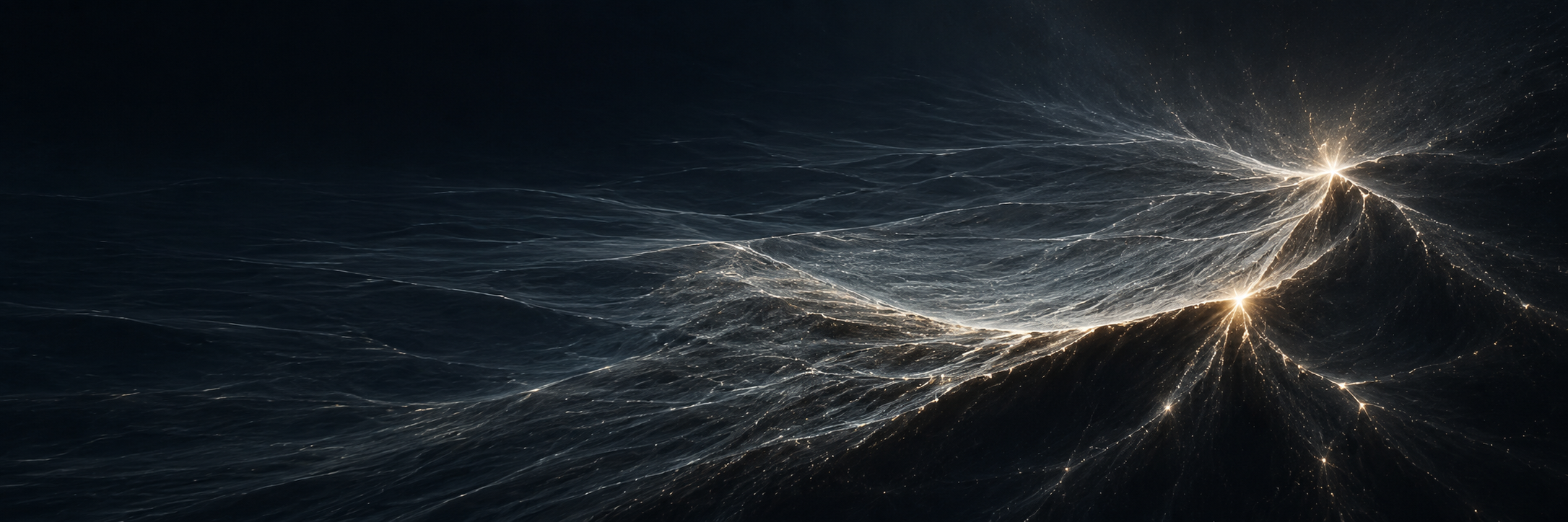
Imagine a universe with no galaxy. Galaxies do not exist yet. It was our universe, thirteen-odd billion years ago: just tiny clumps of matter scattered across a universe that is very nearly featureless.
Nearly. We have an image of that era from the cosmic microwave background—light released when the universe was about four hundred thousand years old. Its temperature varies across the sky by roughly one part in a hundred thousand, and those variations carry the imprint of small unevennesses in the matter — the only relief the young universe had. If the matter field were a landscape, it would be a plain running to every horizon, its ridges and basins so shallow no eye could find them. There are no landmarks. There is nowhere in particular to stand.
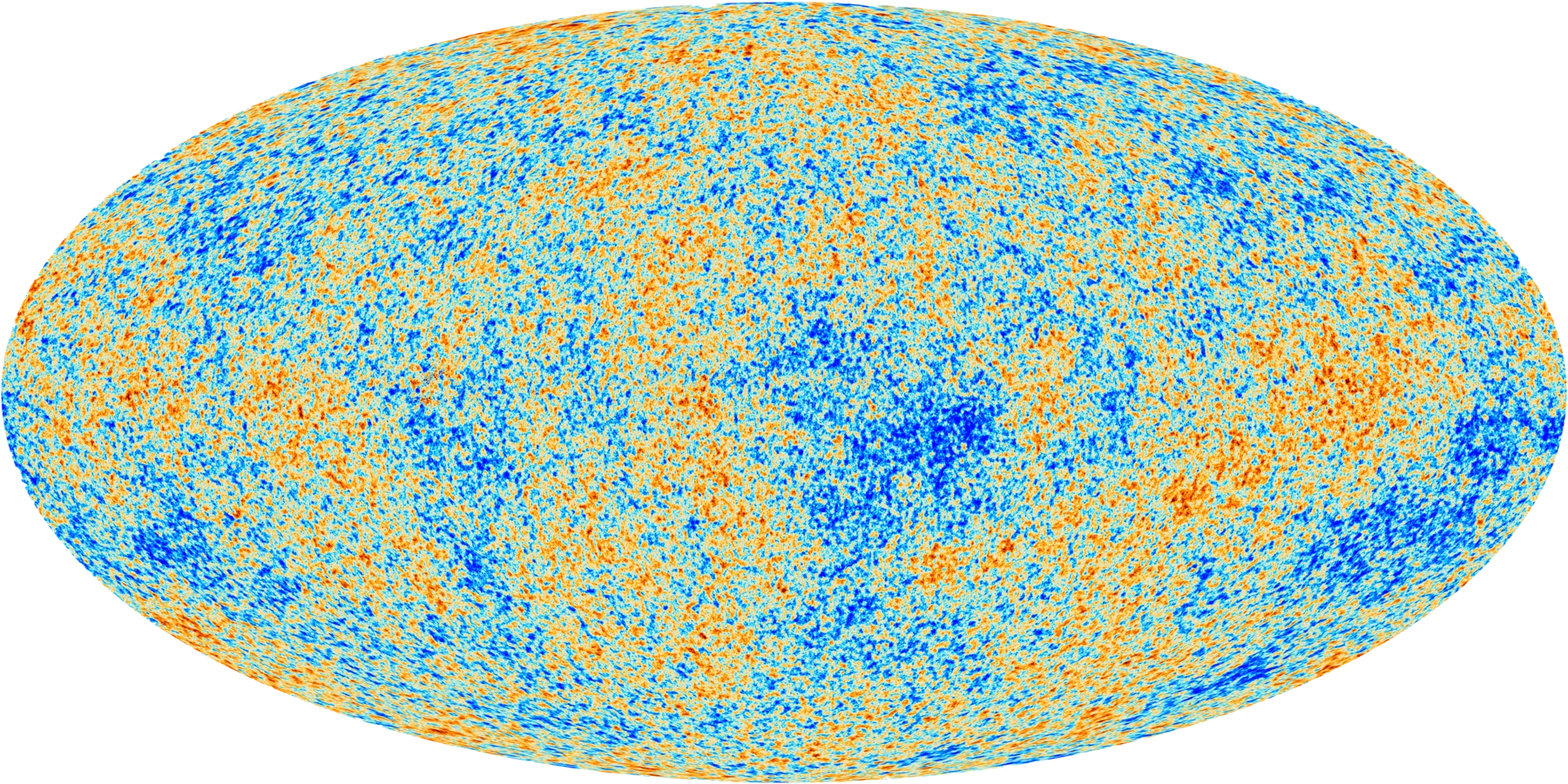
The whole sky, four hundred thousand years in: the Planck 2018 map of the cosmic microwave background. Warmer and cooler spots differ by about one part in a hundred thousand — the buried relief everything below grows from. Credit: ESA/Planck Collaboration. To feel how the cosmological dials reshape this map, try the interactive Planck simulator.
Today the same universe holds the cosmic web: filaments of galaxies strung across hundreds of millions of light-years, dense knots at their crossings, and voids between them so empty they are the emptiest places there are. One of the largest patterns in nature, standing where the plain used to be.
This post is about how you get from one to the other. The answer is not that something drew the web. On the largest scales, gravity does the work: the initial field chooses the geography, and gravity makes that geography visible. And the way it does so — the specific order it works in — is the part almost everyone pictures wrong. I model structure formation for a living, and I pictured it wrong for years.
The smallest advantage
Suppose your parcel sits on one of those shallow ridges — a region holding slightly more matter than average. Slightly is enough. A ridge pulls on its surroundings a little harder than the plain does, so matter drifts toward it. Having gained, it pulls harder still. A slight excess compounds itself. A shallow ridge gains matter and rises; a shallow basin loses matter and empties. Nothing arbitrates this. Gravity has no threshold below which it declines to act; any unevenness, however small, is an instruction to become more uneven.
Notice what the process cannot do. It cannot put a ridge where the initial field put none. It cannot drain a basin that was never there.
Gravity does not draw a new pattern. It raises the contrast of the pattern already present.
Cosmic expansion matters too — the universe stretches the plain while gravity works against the stretch, and their competition sets the pace and how much time the process gets. But the pace is all it sets. The map was drawn at the beginning.
In physical terms, the density contrast grows.
Watch the hidden landscape rise
You can watch this happen. Below is a small universe — 250 megaparsecs of one, computed live in your browser. It opens near the beginning, at one-twentieth of today’s cosmic expansion, rendered as a translucent volume: a pale plain, faintly creased. (The dots you will meet later are tracers of a continuous field, not miniature pieces of cosmic substance.)
Before touching anything, pick one region a shade paler than the rest and commit to a prediction about it. Then press Controls (top right) and, under Cosmic time, press ▶ Grow the universe — holding your eye where you left it.
Nothing enters the box. The existing pattern sharpens. Ridges gather; basins drain. The structure you end with was in the box when you started; you simply could not see it yet.
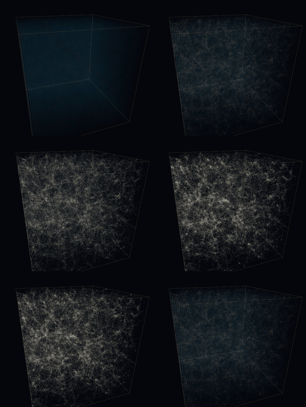
Cosmic time running forward, from a ≈ 0.05 (redshift ~19) to today. Nothing enters the box; the relief that was always there rises until you can see it.
The collapse you pictured is wrong
Now follow your parcel into one of the gathering ridges, because this is where the picture in your head is about to fail.
Here is the picture I carried for years, and the one most people draw: an overdense region contracts toward its center, growing rounder and denser, until it becomes a compact clump. Collapse, in this picture, means falling to a point. It seems too obvious to question — a body of matter falls inward; what else could it do?
Question it anyway. Falling to a point is what a perfectly spherical region would do: contraction at the same rate from every direction at once. And nothing about your parcel’s neighborhood is perfectly spherical. It is a patch of a random field — matter piled slightly deeper on one side, a basin grazing it on another. A random patch has no reason to contract equally in every direction. Whatever it does, it will do unevenly.
So the question “where does the matter go?” becomes a sharper one: along which directions does it go first? That question has an exact answer, and the answer is the whole shape of the cosmic web.
One direction, then two, then three
Stand at your parcel and measure the squeeze. A generic patch of a random field is being compressed at three different rates along three perpendicular directions — a strongest squeeze, a middling one, and a weakest. (You can picture the patch as a slightly flattened ellipsoid if it helps, but the three unequal rates are the load-bearing fact.) The direction with the largest compression reaches collapse first, while the other two are still on their way.
Play it forward. The fastest direction finishes and the patch flattens: collapse along one axis of three. Where a moment ago there was a vague thickening of the plain, there is now a wall — matter drained from two sides onto a surface. Astronomers call these sheets. Zel’dovich, who worked this out in 1970 with little more than the argument you just read, called them by the flatter name the shape deserves.
First a pancake. Then a filament. Only later, a knot.
The collapsing does not stop. Within the sheet, the second direction finishes: the wall drains along itself into a ridge of ridges — a filament, collapse along two axes. And where filaments meet, the third and slowest direction finally arrives, and matter falls in from every remaining side to form a node — collapse along all three, the dense knots where clusters of galaxies live. The point-collapse you pictured does eventually happen. It happens last, and only in the rare places where all three directions have finished.
Watch it happen before we name it. The box below opens early again, with every tracer colored by its collapse state. Ignore the bright knots. Watch what appears first.
What you just watched was a count. At every point, tally how many of the three directions have collapsed, and you have named every environment in the cosmic web: zero, a void; one, a sheet; two, a filament; three, a node. In this dynamical classifier, the four web environments correspond to the number of principal directions undergoing collapse — one modest counting argument underneath this entire taxonomy. That is what I find beautiful here. Not four theories for four kinds of structure: one approximation, one count.
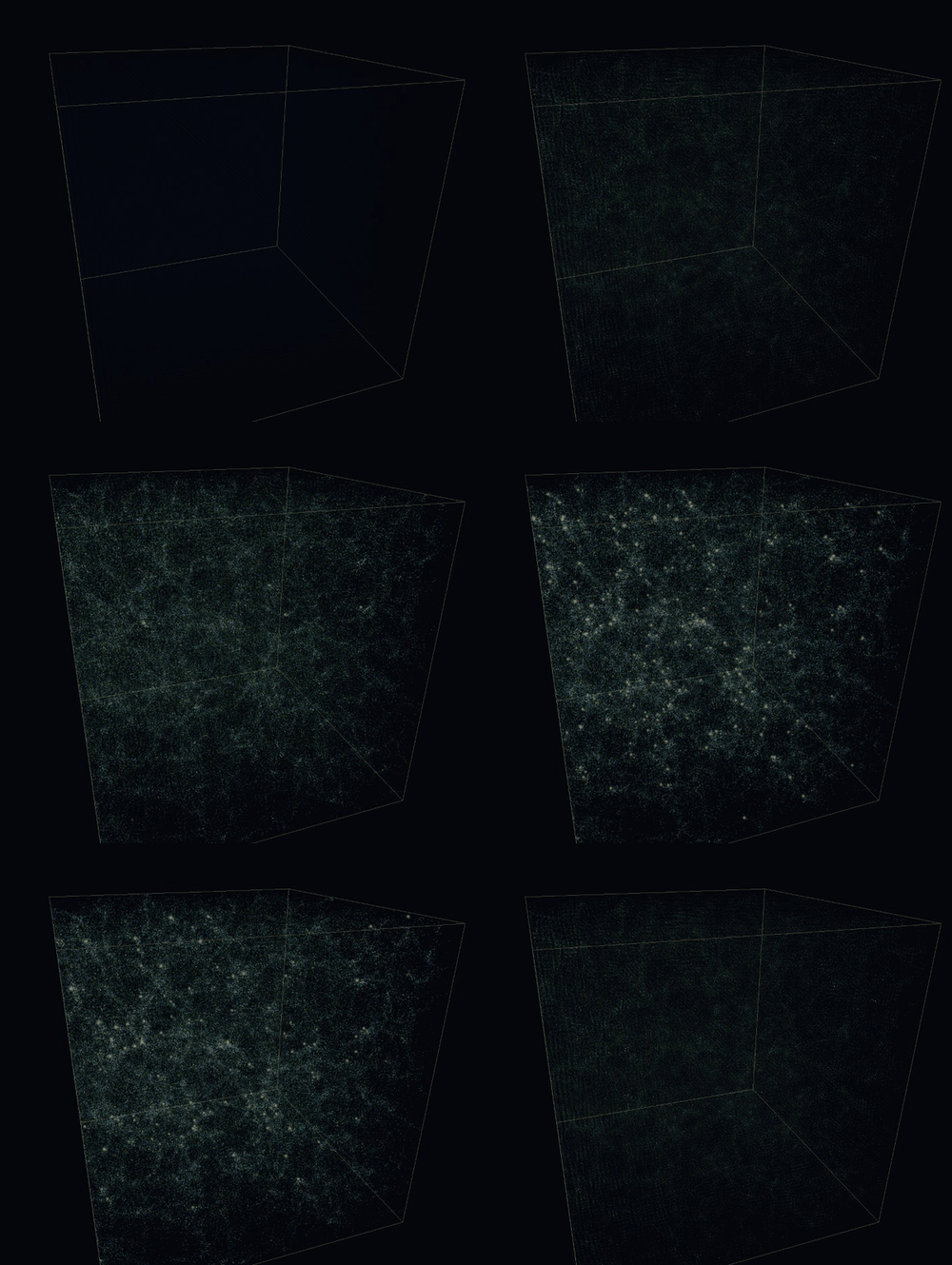
The same growth, each tracer colored by how many of its directions have collapsed: voids dark, sheets green, filaments blue, nodes orange. Flat structures light up first. Knots come last.
Technical interlude — the classifier, precisely
The three compression rates are the eigenvalues λ₁ ≥ λ₂ ≥ λ₃ of the deformation tensor, the 3×3 symmetric gradient of the displacement field Ψ below. A direction counts as collapsed when D(t)·λ crosses a threshold, and the count (0–3) picks the color — a T-web-style dynamical classification, after Forero-Romero et al. (2009): one useful classifier of web environments, not their unique definition. The strict Zel'dovich caustic sits at D·λ = 1, but at that threshold almost no nodes exist by today, so the box uses a gentler one; the ordering is the same either way. The shader solves the cubic characteristic equation in closed form (index.html:651 of the sandbox). For careful derivations of the displacement field and its second-order (2LPT) correction, see Donghui Jeong's PhD thesis, Cosmology with high (z > 1) redshift galaxy surveys (University of Texas at Austin, 2010).
One field and one growing number
Everything so far — the amplification, the three-way collapse, the count — compresses into one line. It is the line the browser universe actually computes, and it deserves to be read slowly.
x(t) = q + D(t) · Ψ(q)
Read it as your parcel’s whole story. q is where you began on the primordial plain. Ψ(q) is a fixed arrow attached to that spot — direction and length prescribed once by the initial field, never redrawn. D(t) is the growth factor: a single number, the same number everywhere in the universe, rising as cosmic time passes. Your position now, x(t), is your origin plus your arrow times that number. That is the Zel’dovich approximation, and it is the whole dynamics: every parcel slides along its own frozen arrow, and the only thing that ever changes is one number.
This is why the geography was never in doubt. The arrows were fixed at the beginning; time only turns the dial that scales them. And the initial ripples in the matter density — ripples in the sense of a pattern of slight excesses and deficits; nothing rolls through space like surf — came with one more property that matters: their initial amplitude determines how much relief gravity has to amplify. In the box below, open Controls; the amplitude is the dial marked σ₈. Sweep it with the realization held fixed and watch what changes and what refuses to: collapse runs further or less far, but the ridges stand exactly where they stood. The primordial field chose the geography. Amplitude mainly sets how far collapse has progressed.
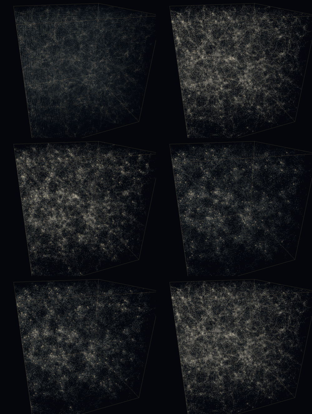
Sweeping σ₈, the amplitude of the initial ripples, with the realization held fixed. Collapse runs further or less far; the ridges stand where they stood. Amplitude mostly sets how far, not where.
Where the vision stops being exact
Honesty about the tool. The Zel’dovich approximation is exact about the question this post asked — which directions collapse, and in what order — and increasingly wrong about what happens deep inside the structures afterwards. Once streams of matter pass through one another — shell crossing, in the trade — real gravity would pull them back; frozen arrows let them keep going. So the sheets and filaments here are real and correctly ordered, while the exact densities inside the brightest knots are not numbers I would put on a plot. (The box offers an optional second-order correction, 2LPT, that sharpens the knots toward the full answer. And one implementation note, since someone always asks: it runs on a fixed random seed, so it is reproducible — every reload is the same universe, and every dial changes the physics rather than the luck of the draw.)
How a laptop solves for the arrows at all — why the calculation collapses to a handful of Fourier transforms, and where the browser gets a power spectrum — is its own story, for a companion post: How to fit a universe in a browser. The full sandbox, with every control this post kept out of your way, is here: open the Cosmic Web Sandbox ⤢.
Technical note — dots, clouds, and where the brightness comes from
Because the dots are tracers of a continuous field, the same physics renders two honest ways: draw the tracers themselves as points, or bin them back into the density they sample and ray-march it as a translucent volume — the cloud view the first encounter opened in.
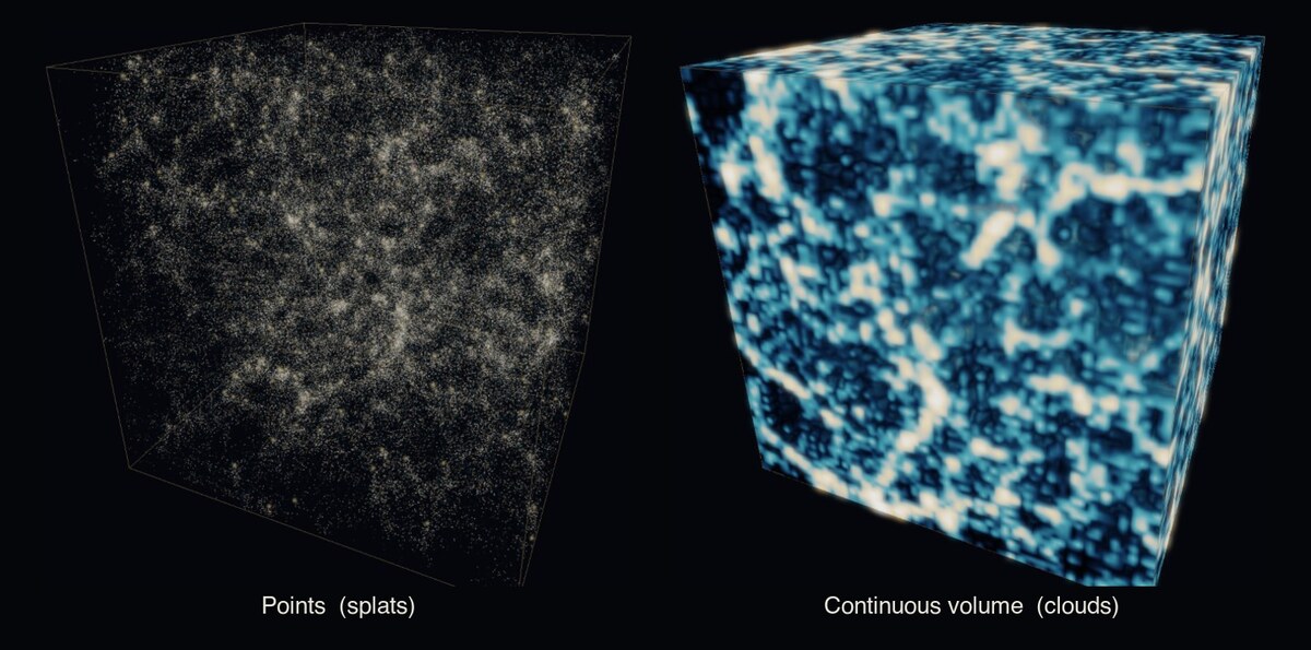
The identical box, same seed and same instant — tracers as points on the left, the continuous density they sample on the right. The points sample the cloud; the cloud is what the points are sampling.
Brightness carries a single-stream density from the Jacobian of the displacement, 1 + δ = 1 / det(I + D·A) — one over how much a fluid element has been stretched (index.html:645). Where that determinant crosses zero, streams pile up in a caustic and the density formally diverges: that is the bright edge lighting a collapsing sheet.
The old pattern, made visible
Go back to the plain one last time — the parcel, the shallow ridge no eye could find. Every structure in tonight’s sky was already there: the wall of galaxies as a slight extra depth of matter, the void as a grazing shallowness, the great cluster as the crossing of three faint creases. Nothing designed the web, and nothing needed to. Gravity took the buried map and raised its contrast, one direction at a time, until the map became legible. Flat first, then thin, then a point.
The universe makes pancakes first, and everything else is patience.